The ULLYSES team produces several types of High Level Science Products (HLSPs), described in detail on this page. Hubble Space Telescope (HST) products are made using both new HST observations obtained through the ULLYSES program as well as archival data. Las Cumbres Observatory (LCO, formerly Las Cumbres Observatory Global Telescope) products are made using LCO observations obtained through the ULLYSES program. VLT HLSPs are created using products provided by the community collaboration groups PENELLOPE and XShootU.
Data products are available from the ULLYSES search form hosted by MAST (HLSPs only), the MAST Data Discovery Portal (HLSPs and contributing data), or directly as a High-Level Science Product collection using the DOI (HLSPs only). Instructions on how to use the MAST Portal can be found here.
Instructions and examples on how to retrieve, use, and create your own data products can be found in the ULLYSES Jupyter Notebooks.
- Data Product Types
- Latest Data Release
- Download Data
- Data Product Creation
- Coadding Spectra with a Common Grating
- Abutting Spectra with Different Gratings and Instruments
- Creating Time-series Spectra
- LCO Data Processing
- FUSE Data Processing
- Correcting COS Wavelength Offsets
- Correcting COS NUV Vignetting
- STIS Recalibration
- STIS Lowest Echelle Orders
- STIS Blaze Correction
- WFC3 Drizzled Images
- Community Data Products
- Data Product Naming Convention
- Data Product Format
- Single-epoch Spectra
- Time-series Spectra
- Community-submitted PENELLOPE Spectra
- Community-submitted XShootU Spectra
- WFC3 Drizzled Images
- YAML files
- Publications
🔗 Data Product Types
The ULLYSES team creates several types of data products, or HLSPs, to maximize the science return of the project. Data from HST/COS, HST/STIS, HST/WFC3, FUSE, and LCO are used. Products are differentiated by their HLSP level identifiers, as follows:
- Level 0: Spectra that have undergone custom calibration outside of the standard pipeline, (for example defringing STIS spectra) and any accompanying calibration paramter files. Level 0 products have the suffix spec.fits or spec.yaml.
- Level 2: Coadded spectra, where the input spectra are of the same instrument and grating. Level 2 products have the suffix cspec.fits.
- Level 3: Abutted level 2 products, grouped by instrument and resolution. For example, all level 2 medium-resolution COS spectra are abutted together into a single spectrum. Level 3 products have the suffix aspec.fits.
- Level 4: Abutted level 2 products, abutting all available spectra regardless of instrument or setting. Level 4 products have the suffix preview-spec.fits, since they are meant for visualization purposes only. The ULLYSES team recommends using level 2 coadded spectra for science purposes.
- Level 5: Time-series spectra for stars whose flux is variable. Level 5 products have the suffix tss.fits and split-tss.fits.
- Level 6: WFC3 drizzled images for two low-metallicity galaxies, Sextans A and NGC3109. Level 6 products have the suffix drc.fits.
- Level 7: Community-contributed VLT spectra of ULLYSES sources. Level 7 products have the suffix vltspec.fits.
🔗 Download Data
Data products are available from the ULLYSES search form hosted by MAST (HLSPs only), the MAST Data Discovery Portal (HLSPs and contributing data), or directly as a High-Level Science Product collection using the DOI (HLSPs only). Instructions on how to use the MAST Portal can be found here.
↑ Jump to top of page
🔗 Data Product Creation
↑ Jump to top of pageSpectra of ULLYSES targets were obtained with multiple observatories, and for each observatory, multiple instruments and/or grating settings were used. Some of the spectra are obtained with an echelle grating, some with single-order small or large aperture, and some with single-order long-slit configurations. The approach for combining data depends upon whether the input spectra share a common instrument and grating. For COS, x1d products are used, not x1dsum products, as x1dsum are created using a linear interpolation method that introduces noise correlation between neighboring output pixels. For all STIS CCD and some single-order MAMA data, custom-calibrated x1d products are created. Otherwise, default x1d products are used. For FUSE data, Virtual Observatory (VO) files are used, and rescaled when necessary. For LCO data, BANZAI pipeline products (McCully et al. 2018) are used. For WFC3 data, default flc files are used to create drizzled products. For all input datasets, custom processing may be applied to correct various detector and observational effects, as described in the following sections.
For each source, the ULLYSES team combines 1) adjacent spectral orders within a single echelle exposure and 2) different exposures obtained with a common grating, using the same or different central wavelength settings. This approach is used to create level 2 cspec.fits files.
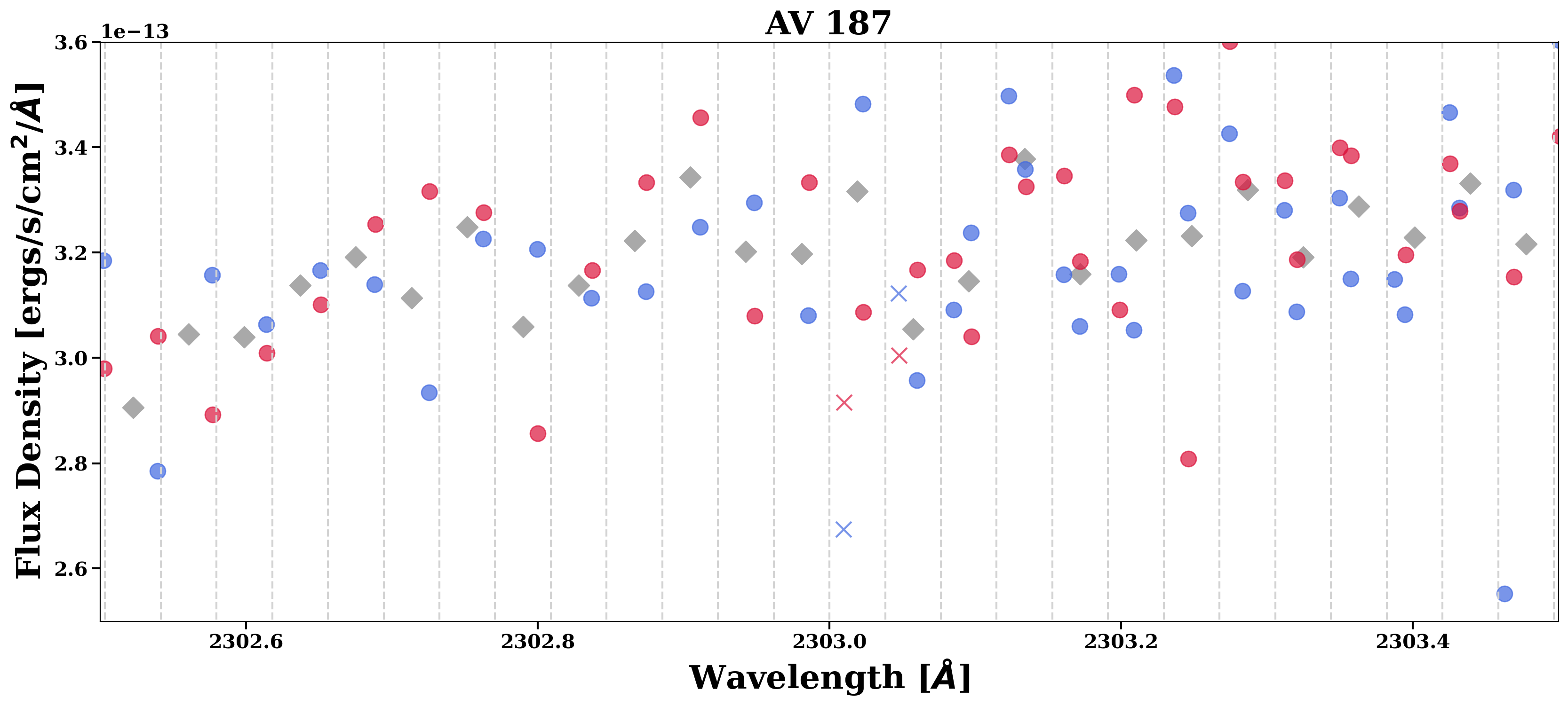
Each input pixel measurement is treated as an estimate of the monochromatic flux at its assigned wavelength. The wavelength bin sizes are constant across the entire wavelength range, where the bin sampling is equal to the coarsest wavelength sampling of all input datasets. The output flux is obtained by calculating a weighted average of all the flux measurements that fall within the output pixel's bounds. The throughput (net count rate divided by flux) times the exposure duration is used as the weighting factor for each input pixel, so that measurements derived from more counts have higher weights. Only input pixels with corresponding Data Quality (DQ) flags that are not considered serious contribute to the output flux. Figure 1 shows an example of how fluxes from two overlapping spectra are mapped to the imposed wavelength grid of the output spectrum.
The error array is calculated as the square root of the total counts that contribute to the output pixel, converting to flux units by multiplying by the flux/net counts at that wavelength. If the net counts and flux are zero, the conversion ratio is interpolated using neighboring values. The signal to noise ratio (SNR) is calculated for each wavelength bin as the ratio of the flux to the error.
This method of combination avoids correlating errors in neighboring pixels, at the cost of a very small loss in spectral sampling.
For each source that has spectra from different gratings, instruments, and/or telescopes, the contributing level 2 cspec.fits spectra are spliced together. This approach is used to create level 3 aspec.fits and level 4 preview-spec.fits products.
For non-overlapping spectra, the arrays are abutted as-is and the spectral sampling will be discontinuous at the transition point(s).
For overlapping spectra, a transition wavelength is selected. The input spectra are truncated and abutted at that wavelength, so the spectral sampling will be discontinuous at the transition. The transition point(s) are determined automatically by the HASP (Hubble Advanced Spectral Products) software that ULLYSES utilizes. For a given source, all contributing gratings have a pre-defined wavelength range within which the data are considered "good". Each grating also has a preassigned priority number. Iterating over all contributing gratings for the full wavelength range, data from the highest priority grating is selected over lower priority gratings. In practice, this is implemented by assigning 2 transition wavelengths to each grating spectrum, one for the shortest wavelength that fits in the fiducial wavelength range, and one for the longest wavelength. The full list of transition wavelengths from each input grating product is then traversed, and at each transition a decision is made as to which grating has the highest priority and will be used until the next transition wavelength. The transitions are abrupt, and the resolution and wavelength spacing will change from grating to grating. While this method works well for most targets, there are a select number of targets where the abutted products might not be ideal. In these rare cases, we encourage use of the level 2 cspec.fits files instead. We emphasize that the level 4 preview-spec.fits products are intended primarily for visual inspection, and level 2 or 3 products should be used for scientific analysis.
↑ Jump to top of sectionExposure-level time-series products are created for survey and monitoring T-Tauri stars. LCO, HST/COS, and HST/STIS data are all used. Sub-exposure-level time-series products are created for monitoring T-Tauri stars only and use only HST/COS data, as that is the only mode where time-tag data can be further split.
Input Data
For all survey and monitoring stars observed by the ULLYSES team, LCO images are taken over five epochs. The first four epochs occur approximately 90 and 10 days before, and 10 and 90 days after, HST observations. Each of these epochs consists of daily observations over a 10-day interval. The fifth epoch occurs during the HST observations, and where LCO images are taken every 15 minutes. Each LCO observation includes back-to-back images in the filters applicable for the star type. Monitoring stars use SDSS u’ and i’ filters as well as the Bessel V filter. Survey stars only use the SDSS i’ and V filters. Unsuccessful observations will cause some gaps in either time or wavelength coverage. LCO “wavelength arrays” are limited to the central wavelengths of each filter. LCO data is used to create exposure-level tss.fits files, and is not obtained for survey stars with purely archival data.
For survey stars, HST exposure-level tss.fits files are created for any sources that 1) have multiple epochs, either through ULLYSES observations or archival observations, and 2) exhibit variability across epochs.
Monitoring T Tauri stars in the ULLYSES program are observed with HST/COS. Each visit is executed in the following order: a COS/G230L/2950 observation, a COS/G230L/2635 observation, COS/G160M/1589 exposures at FP-POS 3 and 4, and COS/G160M/1623 exposures at FP-POS 1 and 2. These observations are taken in two epochs, separated by approximately a year. There are four observations per rotation period, and three rotation periods in each epoch, yielding 24 exposures per target per central wavelength setting. These data are used to both exposure-level tss.fits and sub-exposure-level split-tss.fits files. In addition to this data obtained by the ULLYSES team, any additional archival data of monitoring stars is used to create exposure-level tss.fits files.
Input Data Calibration
For LCO time-series products, aperture photometry and flux calibration are performed on calibrated images. Full details on LCO data calibration are included below.
For exposure-level time-series products using HST data, default x1d files from MAST are generally used as input to the HLSP creation code. When it is required, custom-calibrated spectra may be used, e.g. when custom extraction is needed for STIS data or wavelength offsets are required for COS data.
For sub-exposure time-series products using HST/COS data, default corrtag files files from MAST are split into smaller time bins using the costools.splittag routine. This creates multiple “split corrtags”, each of which is then calibrated using CalCOS to produce individual “split x1d” products.
Time and Wavelength Sampling
The time sampling for exposure-level time-series products is determined by the time of observation of each exposure. Native wavelength sampling is always used for exposure-level time-series spectra (i.e. data are not binned in wavelength).The time and wavelength sampling for sub-exposure time-series spectra is optimized to probe the smallest time interval possible while maintaining a S/N ≥ 5 per resolution element at the peak of the most important emission lines: C IV (1548 Å), and Mg II (2800 Å). For all COS/NUV observations, the optimal time sampling and wavelength sampling were determined to be, respectively, 10s and the native wavelength grid (i.e. no wavelength binning, or ~0.415 Å). For FUV the following time and wavelength bins have been adopted for the four monitoring T Tauri stars:
- TW Hya: time = 30s, wavelength = 3 pixels
- RU Lup: time = 30s, wavelength = 6 pixels
- BP Tau: time = 30s, wavelength = 6 pixels
- GM Aur: time = 90s, wavelength = 6 pixels
The final sampling is chosen to ensure that products are ready for use out-of-the-box and require no additional binning for most science goals. However, if a higher S/N is required, data can be further further in time or wavelength by the user, or use the exposure-level files may be used.
Creation and Format of Time-series Spectra
While the exact method of creating the time-series products differs when using LCO versus HST data, the data formats of the output products are identical.
For LCO data, an ASCII photometric file is used as input— this file includes the LCO image filename, MJD start, MJD stop, central wavelength, flux, and error of each observation. The LCO central wavelength is defined as 3560 Å for the u' filter, 5450 Å for the V filter, and 7670 for the i' filter.
For HST data, default MAST x1d files, or custom-calibrated x1d files, are used as input.
For each time-series spectral product, all input data are rebinned onto the same wavelength grid. The exact wavelength sampling is detailed in the Time and Wavelength Sampling section. Data are then assembled into a 2-D array by inserting each rebinned spectrum into a row of a 2-D image. The X-axis of the image represents wavelength, and Y-axis represents time, with time increasing with increasing Y. The same process is used to create a 2-D image for the flux error. Separate 1-D arrays in the data extension give the wavelength as a function of the column number, and the MJD start and stop times as a function of the row number. An illustration of the 2-D flux array is shown below in Table 1.
For an example of how to read in and explore these products, see the "ULLYSES Walkthrough" Jupyter Notebook section "Time-series spectra".
| Time3 | 0 | 1.5 | 1.0 | 1.0 |
| Time2 | 0 | 1.4 | 1.0 | 1.0 |
| Time1 | 1.0 | 1.3 | 0 | 0 |
| Time0 | 1.0 | 1.2 | 0 | 0 |
| Wavelength0 | Wavelength1 | Wavelength2 | Wavelength3 |
The input for ULLYSES processing of LCO data are the LCO BANZAI products. After ULLYSES calibration of BANZAI products, level 5 exposure-level time-series spectra are produced, with suffix tss.fits.
LCO images reduced with the BANZAI pipeline
(McCully et al. 2018)
are available in the LCO archive (see
DDT2020B,
DDT2021A).
BANZAI performs bad-pixel masking, bias and dark removal, and flat-field correction.
It also determines the astrometric solution and extracts a catalog of sources. Using the
BANZAI-reduced images, an absolute flux calibration is determined based on
magnitudes cataloged by the
AAVSO Photometric All-Sky Survey
(APASS, funded by the Robert Martin Ayers Sciences Fund and NSF AST-1412587).
The ULLYSES LCO calibration pipeline is written in IDL. It first performs
aperture photometry on sources in the BANZAI-generated catalog using
aper.pro from the IDL
Astronomy User's Library
(Landsman 1993).
It sums counts in a five-pixel radius and subtracts the modal signal in an
annulus extending from 10 to 20 pixels. These sources are matched to sources
in the APASS tables, using a matching radius of 2 arcsec. The relationship
between APASS magnitudes and –2.5 times the logarithm of the LCO counts is
fit with a line, ignoring three-sigma outliers. The slope of this line can
vary to account for non-linearity in the instrument response; this term is
typically very close to 1.
Next, the pipeline attempts to find a point source at the expected
coordinates of the ULLYSES target. If a source is found, aperture photometry
is performed using the same parameters described above. The measured counts
are converted to a magnitude with the relationship determined above.
Magnitude is then converted to a flux density using the zero-magnitude flux
for the observed bandpass. Central wavelengths and zero-magnitude fluxes come from
Bessell et al. 1998
for the Bessell V filter and from
Fukugita et. al 1996
for the Sloan Digital Sky Survey (SDSS) i' filter. The uncertainty is assumed
to be dominated by the uncertainty in the measured counts of the ULLYSES target.
Measurements with uncertainties greater than 20% of the fluxes (S/N < 5) are discarded.
Output photometry files are then used as input to the spectral time-series
creation code.
For the u' photometry, there are some differences in the procedure due to the sparseness
of the science fields at this wavelength. Separate calibration fields are observed close
in time and airmass to the science fields. If BANZAI is unable to determine an astrometric
solution for the calibration field, a 500 pixel box is searched for the brightest star
around its expected location, and 200 pixel boxes are searched for additional calibration
stars at their expected offsets from the brightest calibration star. Magnitudes for the
calibration stars at u' are obtained from Version 2.4.2 of STScI's
Guide Star Catalog.
For the science field, each u' image is almost always followed by a V image with no
intervening telescope motion, so the u' astrometry is copied from the subsequent V image.
The flux vs. counts relationship found for the calibration field is applied to the science
target after correction for the different exposure times and airmasses. The airmass
correction, central wavelength, and zero-magnitude flux for the SDSS u' filter come
from Fukugita et. al 1996.
All archival FUSE data used in the ULLYSES sample are examined and vetted by the ULLYSES team. Generally, FUSE Virtual Observatory (VO) files are used with no modification. However, some targets exhibit various issues in their spectra, such as spectral channel drifting. Beginning in DR6, the ULLYSES team began to deliver improved spectra for such targets. These custom-calibrated FUSE spectra are delivered as level 3 aspec.fits products, since FUSE VO files are several individual channel spectra abutted together.
Using the strategy outlined below, FUSE data for 26 targets previously excluded from the sample were able to be rectified and included in data products. Even with extra processing, FUSE data for 4 targets were still unable to be rectified and are not included in the ULLYSES sample:
- PGMW-3120: multiple stars in aperture
- AV-22: multiple stars in aperture
- AV-287: target not in aperture
- SK-69D220: multiple stars in aperture
Flux Differences Due to Guiding
Some ULLYSES FUSE data suffer from drifts among the spectral channels; FUSE was essentially four independent spectrographs and thermal instabilities on orbit could cause each one to drift out of alignment. One of the four channels was used for guiding, and the flux in this channel was generally the most accurate. Usually, thermal drifts in the other channels led the target to drift out of the aperture, resulting in lower count rates and thus spectral fluxes. In crowded fields, these drifts could allow a neighboring star to drift into the aperture, resulting in higher fluxes in the final spectra. The following strategy was used to repair these data:- Begin by examining the VO file, which was initially created by splicing together pieces of the extracted spectra from the eight FUSE detector segments.
- If the VO file does not meet data quality needs (e.g., depressed flux or mismatching flux at channel transition points), a new VO file is created by using the eight individual extracted spectra in the “ALL” files. These eight spectra are shifted to a common wavelength zero point and rescaled to create a new VO file.
- The guide channel is identified (LiF1A for the first half of the mission, and LiF2A for the second) and its spectrum adopted as a reference.
- If the spectra from other channels are less than 50% brighter than the reference, then they are rescaled to match the reference in the region of overlap.
- If they are more than 50% brighter than the reference, they are assumed to be contaminated by nearby stars and not included in the final spectrum.
Background Subtraction Corrections
It was also necessary to run parts of the FUSE calibration pipeline (CalFUSE) in cases where the original background subtraction failed. FUSE did not have a shutter, so the detector received light from all three apertures (LWRS, MDRS, and HIRS) at all times. CalFUSE assumes that only the target aperture contains a star and fits a background model to the rest of the detector. In crowded fields, nearby stars occasionally fell in a non-target aperture, leading to an over-subtraction of the background. In these cases, the region of the detector used to model the background (stored as header keywords in the intermediate data file) was modified, and spectra were re-calibrated. ↑ Jump to top of sectionOccassionally, a star is not exactly centered in the COS 2.5" aperture. When this occurs, there can be systematic offsets in the final wavelength scale. This effect is easily corrected by measuring the offset and supplying it to CalCOS (see Section 5.3.2 of the COS Data Handbook). After correcting offsets, level 0 spec.fits are created.
Four stars in the ULLYSES sample exhibit such COS wavelength offsets:
- LMC079-1: visit le2701
- SZ-10: visits leilac, leil2d, and leilad
- V-GM-AUR: visit lek71f
- V-TW-HYA: visit le9d1c
The COS/NUV channel suffers from vignetting in the shortest wavelengths of each NUV stripe (see Section 5.1 of the COS Data Handbook). For ULLYSES observations of the four monitoring T Tauri stars (V-BP-TAU, V-GM-AUR, V-RU-LUP, V-TW-HYA), vignetting is corrected by scaling the flux in vignetted regions to the flux in the same region with a different COS configuration (that does not suffer from similar vignetting). For all other targets, however, COS/NUV observations lack such overlapping spectra. For these targets, the vignetted regions— defined as the first 200 pixels of each NUV stripe— are flagged and discarded.
For the monitoring stars, the vignetting scaling is performed as part of automated pre-processing of time-series spectra, therefore no corrected spectra for individual exposures are delivered. Instead, the spectra present in the level 5 time-series products includes the vignetting correction.
↑ Jump to top of sectionAll STIS CCD, and some STIS single-order MAMA data, require manual calibration. For these targets, the resulting spectra are delivered as level 0 spec.fits files. All corresponding non-standard calibration parameters are recorded in YAML configuration files, with suffix spec.yaml. Both spec.fits and spec.yaml files are considered level 0 HLSPs.
The following detector and data effects are corrected in STIS level 0 products, and each is described in detail below:
- CCD only: DQ=16 overflagging (pixels having dark rate >5σ times the median dark level)
- CCD only: NIR fringe pattern
- CCD and MAMA: custom extraction(s)
DQ=16 Flagging
When creating ULLYSES HLSPs, all spectral elements with a DQ value considered serious are excluded
when coadding and abutting data.
The DQ=16 flag, which notes pixels having a dark rate >5σ times the median dark level, can affect
more than 5% of STIS/CCD pixels. When a spectrum is extracted, however, very large portions (>30%) of
the spectrum can be marked as DQ=16, due to the boxcar extraction method. The majority of these
flagged spectral elements are indeed good and should be included in data products. To address this
this problem, the ULLYSES team applies a less aggressive dark flagging threshold. This is done by
creating new superdarks with modified DQ arrays. The DQ arrays from the dark are then inherited by
the science images themselves. Using this method, it is possible to reduce the incidence of DQ=16
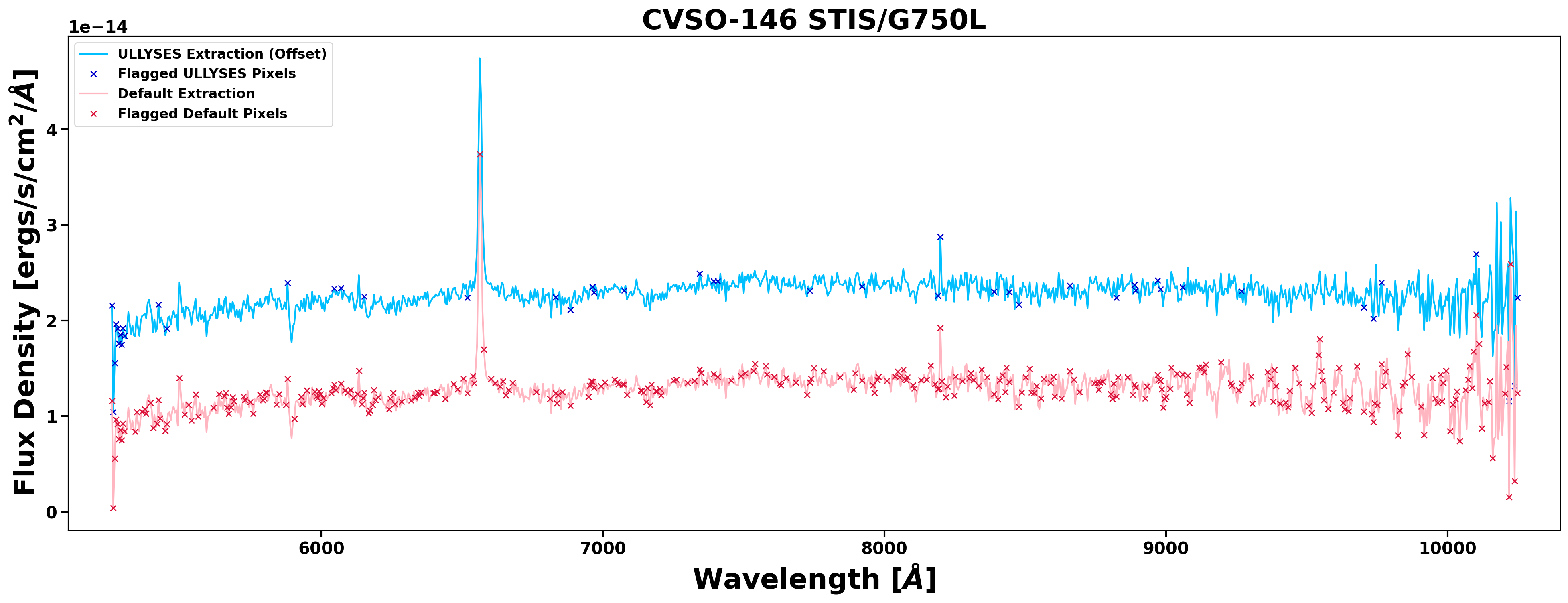
flags by an order of magnitude. See Figure 2 for an example of this improvement.
Defringing
STIS CCD data suffer from an interference pattern called fringing at wavelengths > 7000A, a result of multiple reflections between CCD surfaces (Goudfrooij et al. 1998). Fringing is corrected by obtaining a contemporaneous flat— a fringe flat— using the tungsten lamp and the same grating as the science exposure. For most ULLYSES STIS/G750L exposures, a contemporaneous 0.3x0.09 fringe flat is used. If multiple sources are present in the slit, a contemporaneous 52x0.1 fringe flat may be used instead. If a fringe flat in the appropriate slit was not taken contemporaneously, an archival fringe flat closest to the science observation date is used.
The stistools package defringe tool is used to correct fringing, following the method outlined in the STIS Data Handbook. First, the fringe flat is normalized, then the shifts and scale factors needed to match the fringes in the flat and science spectra are computed. This is often an iterative process; if the best shift and scale values are found at the edge of the supplied range, the range is expanded and the values recomputed. Finally, the science spectra are divided by the scaled and shifted fringe flat. In rare cases, defringing actually degrades the science spectrum quality. For such scenarios, defringing is skipped altogether. See Figure 2 for the comparison between a G750L spectrum with and without fringe correction.
Multiple Sources in SlitThe extraction location and size, cross-dispersion search range, background region locations and sizes, and wavelength offset can all be manually specified when performing a custom spectral extraction.
When multiple sources are present in the slit, multiple, individual, extractions are required. For both ULLSYES source and the "companion" source(s), the following extraction parameters may be modified: extraction location and size, cross-dispersion search range, background region locations and sizes, and wavelength offset. The naming comvention of such companions depends on how close they are to the intended ULLYSES source.
If the ULLYSES source and the companion are close enough to be unresolved in the COS aperture (i.e., they are within 1.25" of each other), three products will be delivered:
- The ULLYSES source only, with the target name in the HLSP filename being
<TARGNAME>A, e.g. CVSO-109A - The companion only, with the target name in the HLSP filename being
<TARGNAME>B, e.g. CVSO-109B - The "blended" source (both ULLYSES and companion flux), with the target name in the HLSP filename being
<TARGNAME>, e.g. CVSO-109
If there is sufficient separation between the ULLYSES and companion source such that they are resolved in the COS separation (i.e., they are separated by more than 1.25"), two products will be delivered.
- The ULLYSES source only, with the target name in the HLSP filename being
<TARGNAME>, e.g. CVSO-104 - The companion only, with the target name in the HLSP filename being the source's catalog name, e.g. GAIA-DR3-3217634157789741952
If the source is poorly centered in the slit, in either the along- or cross-dispersion direction, custom extraction can correct the issue. In most cases, CalSTIS's automatic source location algorithm will successfully extract sources offset in the cross-dispersion direction. However, it may fail for faint sources, and in such cases the extraction location may be manually supplied. When the source is miscentered in the along-dispersion direction, the systematic offset can be calculated and supplied when re-calibrated, rectifying the issue.
Extraction Box SizeSometimes adjusting the extraction box size can result in a higher SNR for the extracted 1D spectrum. In such cases, the height of the extraction box is manually supplied during recalibration.
↑ Jump to top of sectionCalSTIS flags the lowest orders of commonly used echelle configurations as having a poorly determined residual background. However, the fluxes of ULLYSES sources in these orders are accurately determined. To maximize wavelength coverage, the ULLYSES team manually removes the affected Data Quality (DQ) flag, DQ=2048, for these orders only. After removal, the data are included in all subsequent HLSPs. Level 0 spec.fits are also created for these cases.
The affected echelle grating, central wavelength, and orders are:
- E140M/1425 order 86
- E230M/2707 order 66
- E230M/2415 order 73
Misalignments in the STIS echelle blaze function can cause flux mismatches in the overlapping regions of adjacent orders. For a subset of STIS echelle datasets (461 medium-resolution and 11 high-resolution spectra), the ULLYSES team used the stisblazefix tool to empirically correct for such misalignments.
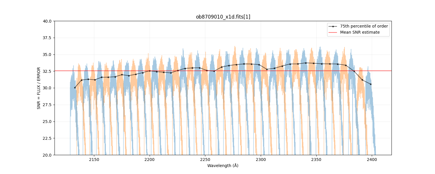
This correction empirically adjusts the alignment of the blaze function by minimizing discrepancies in the overlapping flux of neighboring orders. The linear fit to the applied shift sometimes converges on a false solution, so further inspection is required in the signal-to-noise (SNR) regime where stisblazefix gives reliable results. To do so, the STIS echelle datasets are parameterized by their SNR, and subsampled high-SNR calibration datasets from the STIS MAMA Spectroscopic Sensitivity and Focus Monitor (from Cycle 7-31), to determine the behavior of the algorithm at lower SNR. Only datasets with nonzero exposure time and a "NORMAL" exposure interruption indicator flag (sci_expflag in MAST) are used. Additionaly, some datasets were excluded; OE5CE4010, OE5CE4050, O3ZX050D0, and O3ZX050E0 exhibited issues in their target acquisitions, and O4LU01060 was obtained during a detector power reset. This resulted in a test sample of 225 high-resolution and 236 medium-resolution echelle observations of the white dwarf flux standards BD+28D4211, BD+75D325, and G191-B2B/G191B2B. Datasets were obtained from 1997-09-15 to 2023-09-28. This final suite of data was used to determine the SNR limits to apply to the ULLYSES sample.The average continuum SNR of each echelle x1d dataset was then calculated as follows: dividing the flux by the error, excluding the and first and last 100 pixels from each order, calculating the 75th percentile value for each order, and finally taking the mean across all orders. This proved to be robust to emission and absorption lines, and to the blaze function edges. See Figure 3 for an example SNR estimate.
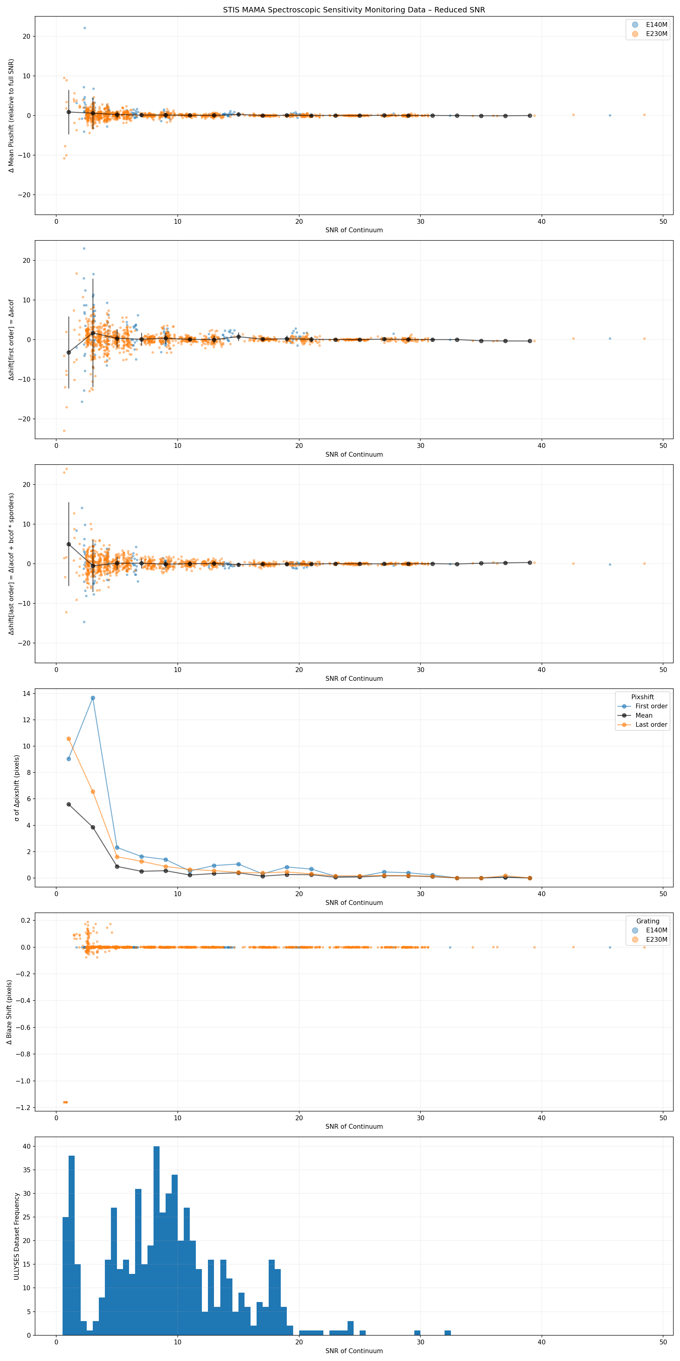
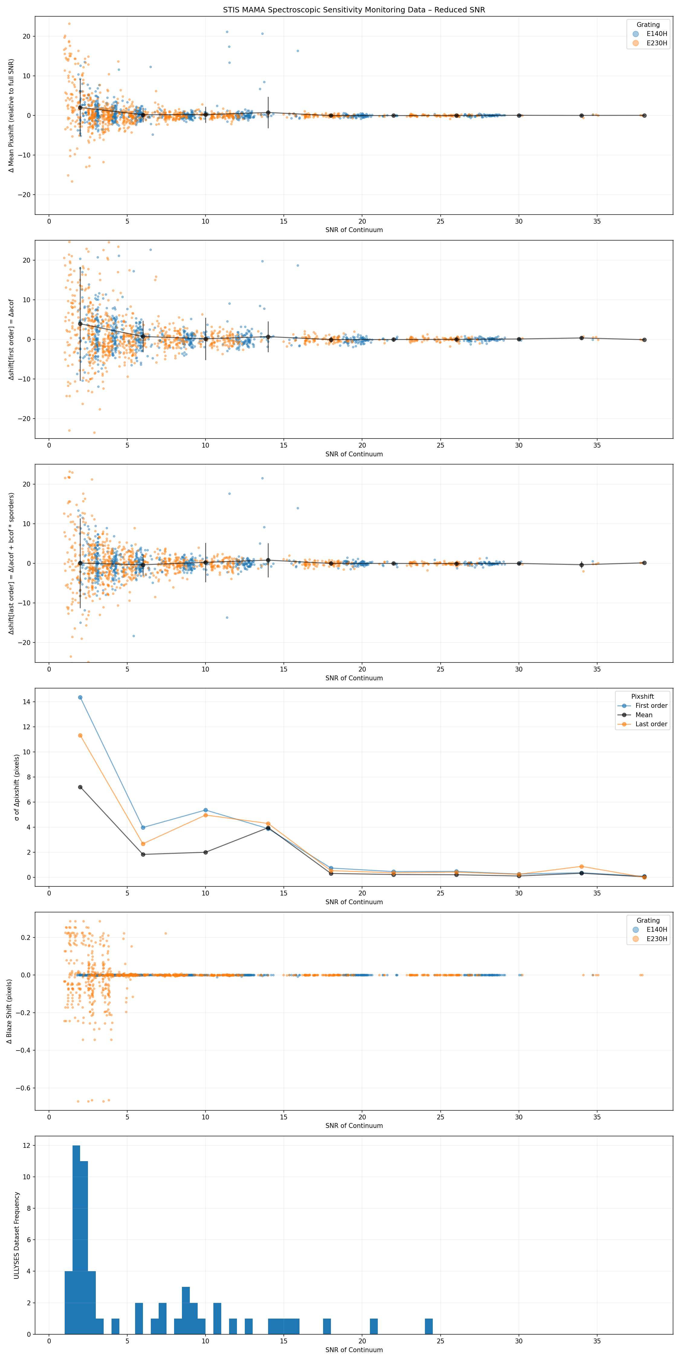
The the monitor datasets were subsampled at levels of [0.5, 1, 2, 5, 10, 25, 50]%, giving a range of continuum flux levels and hence SNR. The subsampled datasets were processed with CalSTIS and stisblazefix to derive the blaze shift offset at the end orders and the mean across all orders. These values are subtracted from those derived from the corresponding full dataset. A more detailed analysis may wish to derive additional data points from more subsamples of the input datasets, especially at lower SNR levels.
When plotted against SNR (see Figures 4 and 5), the scatter in the stisblazefix mean blaze correction increases to ~3 pixel at SNR=10 for H-modes and >2 pixels at SNR=5 for the M-modes. These thresholds also conservatively correspond to a sudden increase in scatter of the calstis-calculated blaze shift value (Δ in the SCI ext "BLZSHIFT" keyword). These SNR thresholds are them used when determining which ULLYSES datasets should be corrected with stisblazefix. Additionally, the stisblazefix diagnostic plots were manually reviewed for obvious bad fits, but nothing was rejected. For M-mode data we used an SNR=5 threshold to apply stisblazefix to 461/590 ULLYSES datasets. For H-mode data we used an SNR=10 threshold to apply it to 11/66 ULLYSES datasets. For each datasets that had stisblazefix applied, all corresponding ULLYSES HLSPs have
COMMENT keywords (in the SCI extension) noting so.
The ULLYSES program obtained spectra of six massive stars in the low-metallicity galaxies Sextans A and NGC 3109. To estimate the exposure time of these stars, pre-imaging, using the HST Wide Field Camera 3 (WFC3) was obtained, using filters F225W, F275W, F336W, F475W, and F814W. Drizzled combined images for each galaxy and filter are delivered as level 6 drc.fits files.
↑ Jump to top of sectionTo fully capitalize on the legacy of the ULLYSES data sample, the ULLYSES team delivered community-created data products from two large external research groups: PENELLOPE and X-Shooting ULLYSES (XShootU). Both collaborations obtained complimentary data of ULLYSES stars using VLT. Community-submitted products are delivered as level 7 prodducts with suffix vltspec.fits.
The PENELLOPE collaboration obtained VLT data of T Tauri stars in the ULLYSES sample, including non-flux-calibrated high-resolution optical spectra (ESPRESSO and UVES instruments) and flux-calibrated medium-resolution UV-to-NIR spectra (X-Shooter instrument). X-Shooter data of 74 T Tauri stars was delivered as ULLYSES level 7 products in early 2024. While the contents of the data arrays were not modified, the original spectra from the three X-Shooter arms (UVB, VIS, NIR) are stored as three separate FITS files by the PENELLOPE team. While the ULLYSES team did not modify the contents of the data arrays in these files, the three files are combined into a single FITS file, with the spectrum (and associated header) of each arm stored in a separate BinTableHDU data extension. The 0th header follows the same format used by all other ULLYSES HLSPs, as is required by MAST HLSP guidelines. Finally, a PROVENANCE BinTableHDU extension, following the same format as all other ULLYSES HLSPs, is added after all data extensions (as a 4th extension).
The XShootU collaboration obtained VLT X-Shooter data of massive stars in the ULLYSES sample. This includes flux-calibrated medium-resolution optical and NIR spectra of 129 LMC stars, 103 SMC stars, and 3 low-metallicity stars. This data will be delivered as ULLYSES HLSPs in the near future.
↑ Jump to top of section
🔗 Data Product Naming Convention
The file names for ULLYSES data products follow a naming scheme which encodes the target name and observing configuration(s) that contribute to the product. Please note that not all products will appear in early data releases. File names have the form:
hlsp_ullyses_<telescope>_<instrument>_<target>_<opt_elem>_<version>_<product-type>
where
- <target> is the target's HLSP name, which can differ from other common aliases due to character restrictions
- <version> is the data release identifier (dr1, dr2, etc.)
The <telescope>, <instrument>, <opt_elem>, and <product-type> templates take names from the following table:
| Description | Telescope | Instrument | Opt-Elem | Product-Type | HLSP Level |
|---|---|---|---|---|---|
| Custom calibrated STIS 1D spectra | hst | stis | g230l | spec.fits | 0 |
| g430l | |||||
| g750l | |||||
| STIS custom calibration parameter files | hst | stis | g230l | spec.yaml | 0 |
| g430l | |||||
| g750l | |||||
| STIS echelle single grating, where the orders have been
extracted and merged. No level 1 products exist. |
hst | stis | e140h | mspec.fits | 1 |
| e230h | |||||
| e140m | |||||
| e230m | |||||
| Combined spectra, with common instrument and grating, and in some cases with different cenwave settings. | hst | cos | g130m | cspec.fits | 2 |
| cos | g160m | ||||
| cos | g185m | ||||
| cos | g230l | ||||
| stis | e140h | ||||
| stis | e140m | ||||
| stis | e230h | ||||
| stis | e230m | ||||
| stis | g230l | ||||
| stis | g430l | ||||
| stis | g750l | ||||
| Combined spectra, with common instrument, different gratings and cenwave settings, and grouped by resolution^ | fuse | fuv | lwrs or mdrs | aspec.fits^ | 3 |
| hst | cos | g130m-g160m-g185m | |||
| stis | e140h-e230h | ||||
| stis | e140m-e230m | ||||
| stis | g230l-g430l-g750l | ||||
| All instruments and settings abutted together* | hst | cos-stis | uv | preview-spec.fits* | 4 |
| cos-stis | uv-opt | ||||
| hst-fuse | fuse-cos-stis | uv-opt | |||
| Exposure-level time-series spectra† | hst | cos | g130m | tss.fits | 5 |
| g160m | |||||
| lcogt† | 04m | v-ip | |||
| Subexposure-level time-series spectra | hst | cos | g130m | split-tss.fits | 5 |
| g160m | |||||
| WFC3 drizzled images | hst | wfc3 | f225w | drc.fits | 6 |
| f275w | |||||
| f336w | |||||
| f475w | |||||
| f814w | |||||
| Community-submitted products | vlt | xshooter | uvb-vis-nir | vltspec.fits | 7 |
| uvb-vis |
* The preview-spec extension was previously named sed prior
to Dec. 14 2021.
^ The aspec extension for level 3 products only was previously named
cspec prior to Dec. 12 2023. It was renamed to aspec to avoid confusion
with the level 2 products which already use the cspec extension.
† At the time ULLYSES LCO products were created, the observatory was known as
LCOGT.
🔗 Data Product Format
↑ Jump to top of pageMost ULLYSES data products are in FITS format. The structure of each FITS file depends on the HLSP type. There are three broad categories of HLSPs: single-epoch spectra, time-series spectra, and drizzled images.
FITS File Structure
Spectral data and information is stored in two BINTABLE extensions:
- a Science extension for the combined product, and
- a matching Provenance extension to record attributes of each spectrum that contributed to the combined product
| Primary Header | Metadata common to all contributing spectra |
| Extension 1 Header | Metadata specific to science
|
| Table 1 Data | Science data specific to single-epoch spectrum |
| Extension 2 Header | Metadata specific to provenance
|
| Table 2 Data | Metadata specific to contributing spectra |
Single-epoch Science Table
Various elements of a single spectrum of M wavelength bins are stored in a single table row; each element is stored in a separate field (i.e., column). The table extension headers also contain informative metadata.
| Column Name | Dimensions | Units | Data Type |
|---|---|---|---|
| WAVELENGTH | M | Angstrom | single-precision float |
| FLUX | M | erg/cm2/s/Angstrom | single-precision float |
| ERROR | M | erg/cm2/s/Angstrom | single-precision float |
| SNR | M | — | single-precision float |
| EFF_EXPTIME | M | s | single-precision float |
Single-epoch Provenance Table
Select metadata for each spectrum that contributes to the combined spectrum in the SCIENCE extension will populate a row in the provenance table. The fields in the following table are metadata harvested from the headers of the contributing spectra.
| Column Name | Units | Data Type |
|---|---|---|
| FILENAME | — | string |
| PROPOSID | — | string |
| TELESCOPE | — | string |
| INSTRUMENT | — | string |
| DETECTOR | — | string |
| DISPERSER | — | string |
| FILTER | — | string |
| CENWAVE | — | string |
| MINWAVE | Angstrom | double-precision float |
| MAXWAVE | Angstrom | double-precision float |
| APERTURE | — | string |
| SPECRES | — | double-precision float |
| CAL_VER | — | string |
| MJD_BEG | d | double-precision float |
| MJD_MID | d | double-precision float |
| MJD_END | d | double-precision float |
| XPOSURE | s | double-precision float |
Time-series Spectra File Structure
Spectral data and information is stored in two BINTABLE extensions:
- a Science extension for the combined product, and
- a matching Provenance extension to record attributes of each spectrum that contributed to the combined product
| Primary Header | Metadata common to all contributing spectra |
| Extension 1 Header | Metadata specific to science
|
| Table 1 Data | Science data specific to multi-epoch spectra |
| Extension 2 Header | Metadata specific to provenance
|
| Table 2 Data | Metadata specific to contributing spectra |
Time-series Spectra Science Table
The time-series spectral products have slightly different table columns compared to single-epoch spectra. The FLUX and ERROR arrays are 2D arrays with wavelength increasing along X, and time increasing along Y. The wavelength values for each column of the 2D data are stored in the WAVELENGTH array, while the MJDSTART and MJDEND columns store the start and end times for each row of the FLUX and ERROR arrays.
| Column Name | Dimensions | Units | Data Type |
|---|---|---|---|
| MJDSTART | M | d | double-precision float |
| MJDEND | M | d | double-precision float |
| WAVELENGTH | N | Angstrom | single-precision float |
| FLUX | M x N | erg/cm2/s/Angstrom | single-precision float |
| ERROR | M x N | erg/cm2/s/Angstrom | single-precision float |
Time-series Spectra Provenance Table
Select metadata for each spectrum that contributes to the time-series product will populate a row in the provenance table. The fields in the following table are metadata harvested from the headers of the contributing spectra. Some columns are only present for HST data or LCO data.
| Column Name | Units | Data Type |
|---|---|---|
| FILENAME | — | string |
| PROPOSID | — | string |
| TELESCOPE | — | string |
| INSTRUMENT | — | string |
| DETECTOR | — | string |
| DISPERSER (HST data only) | — | string |
| FILTER (LCO data only) | — | string |
| CENWAVE (HST data only) | — | string |
| MINWAVE (HST data only) | Angstrom | double-precision float |
| MAXWAVE (HST data only) | Angstrom | double-precision float |
| APERTURE | — | string |
| SPECRES (HST data only) | — | double-precision float |
| CAL_VER | — | string |
| MJD_BEG | d | double-precision float |
| MJD_MID | d | double-precision float |
| MJD_END | d | double-precision float |
| XPOSURE | s | double-precision float |
FITS File Structure
For a complete description of the original PENELLOPE data products, see the ESO release information. Spectral data and information is stored in four BINTABLE extensions:
- a UVB extension for the UVB arm spectra
- a VIS_TELL extension for the VIS arm spectra
- a NIR_TELL extension for the NIR arm spectra, and
- a matching Provenance extension to record attributes of each spectrum that contributed to the final product
| Primary Header | Metadata common to all contributing spectra |
| Extension 1 Header | Metadata specific to UVB spectra
|
| Table 1 Data | Science data specific to UVB spectra |
| Extension 2 Header | Metadata specific to VIS spectra
|
| Table 2 Data | Science data specific to VIS spectra |
| Extension 3 Header | Metadata specific to NIR spectra
|
| Table 3 Data | Science data specific to NIR spectra |
| Extension 4 Header | Metadata specific to provenance
|
| Table 4 Data | Metadata specific to contributing spectra |
PENELLOPE Science Tables
The following science table format applies to the UVB, VIS, and NIR data extensions. Various elements of a single spectrum of M wavelength bins are stored in a single table row; each element is stored in a separate field (i.e., column). The table extension headers also contain informative metadata.
| Column Name | Dimensions | Units | Data Type |
|---|---|---|---|
| WAVELENGTH_AIR | M | Angstrom | single-precision float |
| FLUX | M | erg/cm2/s/Angstrom | single-precision float |
| ERR | M | erg/cm2/s/Angstrom | single-precision float |
| QUAL | M | — | single-precision float |
PENELLOPE Provenance Table
Select metadata for each spectrum that contributes to the the science extensions will populate a row in the provenance table. The fields in the following table are metadata harvested from the headers of the original PENELLOPE products.
| Column Name | Units | Data Type |
|---|---|---|
| FILENAME | — | string |
| PROPOSID | — | string |
| TELESCOPE | — | string |
| INSTRUMENT | — | string |
| DETECTOR | — | string |
| DISPERSER | — | string |
| CENWAVE | — | string |
| MINWAVE | Angstrom | double-precision float |
| MAXWAVE | Angstrom | double-precision float |
| APERTURE | — | string |
| SPECRES | — | double-precision float |
| CAL_VER | — | string |
| MJD_BEG | d | double-precision float |
| MJD_MID | d | double-precision float |
| MJD_END | d | double-precision float |
| XPOSURE | s | double-precision float |
FITS File Structure
For a complete description of the original XShootU data products, see the ESO release information. Spectral data and information is stored in three or more BINTABLE extensions:
- a UVB extension for each UVB arm spectra
- a VIS extension for each VIS arm spectra, and
- a matching Provenance extension to record attributes of each spectrum that contributed to the final product
| Primary Header | Metadata common to all contributing spectra |
| Extension 1 Header | Metadata specific to UVB spectra
|
| Table 1 Data | Science data specific to UVB spectra |
| Extension 2 Header | Metadata specific to VIS spectra
|
| Table 2 Data | Science data specific to VIS spectra |
| Extension 3 Header | Metadata specific to provenance
|
| Table 3 Data | Metadata specific to contributing spectra |
XShootU Science Tables
The following science table format applies to the UVB, and VIS data extensions. Various elements of a single spectrum of M wavelength bins are stored in a single table row; each element is stored in a separate field (i.e., column). The table extension headers also contain informative metadata.
| Column Name | Dimensions | Units | Data Type |
|---|---|---|---|
| WAVELENGTH | M | Angstrom | double-precision float |
| WAVELENGTH_AIR | M | Angstrom | double-precision float |
| SCI_FLUX | M | erg/cm2/s/Angstrom | single-precision float |
| SCI_FLUX_ERR | M | erg/cm2/s/Angstrom | single-precision float |
| SCI_FLUX_QUAL | M | — | single-precision integer |
| SCI_FADU | M | ADU | single-precision float |
| SCI_FADU_ERR | M | ADU | single-precision float |
| SKY_FADU | M | ADU | single-precision float |
| SKY_FADU_ERR | M | ADU | single-precision float |
| SCI_FLUX_SLC | M | erg/cm2/s/Angstrom | single-precision float |
| SCI_FLUX_SLC_ERR | M | erg/cm2/s/Angstrom | single-precision float |
| SCI_FLUX_TAC | M | erg/cm2/s/Angstrom | single-precision float |
| SCI_FLUX_TAC_ERR | M | erg/cm2/s/Angstrom | single-precision float |
| TELLURIC_SPECTRUM | M | — | single-precision float |
| SCI_FLUX_ABS | M | erg/cm2/s/Angstrom | single-precision float |
| SCI_FLUX_ABS_ERR | M | erg/cm2/s/Angstrom | single-precision float |
| SCI_FLUX_NORM | M | — | single-precision float |
| SCI_FLUX_NORM_ERR | M | — | single-precision float |
XShootU Provenance Table
Select metadata for each spectrum that contributes to the the science extensions will populate a row in the provenance table. The fields in the following table are metadata harvested from the headers of the original XShootU products.
| Column Name | Units | Data Type |
|---|---|---|
| FILENAME | — | string |
| PROPOSID | — | string |
| TELESCOPE | — | string |
| INSTRUMENT | — | string |
| DETECTOR | — | string |
| DISPERSER | — | string |
| CENWAVE | — | string |
| MINWAVE | Angstrom | double-precision float |
| MAXWAVE | Angstrom | double-precision float |
| APERTURE | — | string |
| SPECRES | — | double-precision float |
| CAL_VER | — | string |
| MJD_BEG | d | double-precision float |
| MJD_MID | d | double-precision float |
| MJD_END | d | double-precision float |
| XPOSURE | s | double-precision float |
FITS File Structure
Drizzled and weight images are stored in two IMAGEHDU extensions, and PROVENANCE information stored in a BINTABLE extension:
- a Science extension for the drizzled science image
- a Weight extension for the weight map image
- a matching Provenance extension to record attributes of each image that contributed to the combined product
| Primary Header | Metadata common to all contributing images |
| Extension 1 Header | Metadata specific to drizzled science images
|
| Image 1 Data | Drizzled science image |
| Extension 2 Header | Metadata specific to drizzled images
|
| Image 2 Data | Weight map image |
| Extension 3 Header | Metadata specific to provenance
|
| Table 3 Data | Metadata specific to contributing images |
Drizzled Image Provenance Table
Select metadata for each image that contributes to the drizzled image in will populate a row in the provenance table. The fields in the following table are metadata harvested from the headers of the contributing images.
| Column Name | Units | Data Type |
|---|---|---|
| FILENAME | — | string |
| PROPOSID | — | string |
| TELESCOPE | — | string |
| INSTRUMENT | — | string |
| DETECTOR | — | string |
| FILTER | — | string |
| APERTURE | — | string |
| CAL_VER | — | string |
| MJD_BEG | d | double-precision float |
| MJD_MID | d | double-precision float |
| MJD_END | d | double-precision float |
| XPOSURE | s | double-precision float |
All STIS CCD, and some STIS single-order MAMA data, of require tailored calibration. For these targets, all non-standard calibration parameters are recorded in YAML configuration files that are included with ULLYSES data relases. YAML files are considered level 0 products.
↑ Jump to top of section
🔗 Publications
A description of the ULLYSES program, design, and initial results is given in:
For more information on how to cite ULLYSES data, see ULLYSES References.
↑ Jump to top of page