August 31, 2021
Data Release 3 (DR3) consists of high-level science products (HLSPs) for 90 new ULLYSES targets and updated HLSPs for 137 targets previously released in DRs 1 and 2, for a total of 227 ULLYSES targets to date. Updated HLSPs for previously delivered products include recent pipeline and calibration improvements- any existing HLSPs from previous DRs should be replaced with newly downloaded products. HLSPs are also provided for 6 companion targets present in STIS long-slit observations. DR3 includes two new product types – time-series spectra and WFC3 drizzled images – and introduces LCOGT (Las Cumbres Observatory Global Telescope) data for an initial subset of ULLYSES T Tauri stars.- DR3 Target Breakdown
- Updated Massive Star Information
- T Tauri Star Companions
- WFC3 Drizzled Images
- Time Series Spectra
- LCOGT Data
- Targets Requiring Special Calibration
- DR3 Updates to the HLSP Creation Code
- DR3 Caveats and Known Issues
- Download Data
- Publications
DR3 Target Breakdown
227 ULLYSES targets:- 179 massive stars from the LMC and SMC - 55 new to DR3
- All 180 massive stars have HST/COS and/or HST/STIS spectra
- 99 massive stars also have FUSE spectra
- 47 Survey T Tauri stars- 34 new to DR3
- 6 of the stars have only HST COS/FUV and/or STIS/FUV spectra
- 14 of the stars have only HST COS/FUV and STIS/NUV spectra
- 13 of the stars also have LCOGT data
- 27 of the stars have HST COS/FUV, STIS/NUV, and STIS/Optical spectra
- 1 Monitoring T Tauri star (V-TW-HYA)- new to DR3
- Monitoring star has HST COS/FUV and COS/NUV spectra
- These targets are present in STIS long-slit observations of T Tauri stars
- HLSPs for these companions may be used to help de-contaminate unresolved observations of the corresponding T Tauri stars
Updated Massive Star Information
A new CSV file with updated metadata for massive stars, including references, is now available for download here. An HTML table, with hyperlinked references, is also available for download here.T Tauri Star Companions
One survey T Tauri star new to DR3 had two companion sources in the STIS slit, outlined below. For DR2 T Tauri stars with companions, see the DR2 release notes.- 2MASSJ11432669-7804454: 2 unexpected companions. The first companion was identified as GAIA-DR3-5200232636905785728, located approximately 14.66” away from the ULLYSES target. The GAIA identifier was adopted as this companion’s name. The second companion, located approximately 0.165” away from the ULLYSES target, is not in any catalogue to date. The second companion is unresolved in both the STIS and COS apertures. Although no HLSPs are produced for this second companion alone, it is referred to it as 2MASSJ11432669-7804454B. The ULLYSES target plus this second companion together are referred to as 2MASSJ11432669-7804454. Please be advised that all HLSPs for 2MASSJ11432669-7804454 actually include the spectrum from this second, unexpected companion.
WFC3 Drizzled Images
WFC3 drizzled images of the low-metallicity galaxy NGC3109 were previously included on the ULLYSES website for download. In DR3, these images are repackaged as official HLSPs, which are now available through MAST alongside all other ULLYSES HLSPs. These new HLSPs have the extension “_drc.fits” and are defined as level 6 HLSPs.Time-series Spectra
Spectroscopic time-series products are now available for both survey and monitoring T Tauri stars. For survey stars, only exposure level time-series with LCOGT data (with extension “_tss.fits”) are available. HST COS and STIS UV data are time-tagged, which allows for sub-exposure time-series spectra. Sub-exposure products (with extension “_split-tss.fits”) are only generated from HST data of monitoring stars, in addition to exposure level time-series. Both sub-exposure and exposure level time-series are defined as level 5 HLSPs. The data formats of all products are identical for both survey and monitoring stars, but the input data and exact methods of creation differ, as detailed below.Input Data
Both HST and LCOGT data are used to create spectral time-series products.LCOGT data are used to create exposure-level time-series products only. LCOGT time-series products are created for both survey and monitoring stars. Images are taken approximately 90 and 10 days before, during, and 10 and 90 days after HST observations. Full details on LCOGT observations are included below. In DR3, LCOGT products are only created for the 13 survey stars in Orion that were previously released in DR2. LCOGT products for monitoring stars and additional survey stars will be available in the future.
HST data are used to create both exposure-level and sub-exposure-level time-series products. HST time-series products are only created for monitoring targets.
Monitoring T Tauri stars in the ULLYSES program are observed with HST COS/G160M/(1589,1623) and COS/G230L/(2635,2950). Targets are observed with each setting a total of 24 times. These observations are taken in two epochs, separated by approximately a year. There are four observations per rotation period, and three rotation periods in each epoch. DR3 includes the first epoch of spectral time-series products for the first of four monitoring stars, TW Hydra. We will provide additional products for TW Hydra in the future when the second epoch has been completed. One visit (1K) failed, therefore only 11 of the expected 12 visits are available.
Input Data Calibration
For LCOGT time-series products, aperture photometry and flux calibration are performed on calibrated images. Full details on LCOGT data calibration are included below. Only exposure level products are created with LCOGT data.For exposure-level time-series products using HST data, default x1d files from MAST are used as input to the HLSP creation code. For TW Hydra however, special calibration was required to address some issues.
For sub-exposure time-series products using HST data, default corrtag files from MAST are split into smaller time bins using the costools.splittag routine. This creates multiple “split corrtags”, each of which is then calibrated using CalCOS to produce individual “split x1d” products. Again, special calibration was necessary for TW Hydra such that default MAST corrtags could not be used.
Time and Wavelength Sampling
LCOGT images are taken over four epochs, each consisting of daily observations over 10-day intervals. In addition, 15-minute cadence observations are also taken during the HST observations. For each daily observation, back-to-back images are taken in the applicable filters for the star type. Monitoring stars use SDSS u’ and i’ filters and the Bessel V filter, while survey stars only use the i’ and V filters. Unsuccessful observations will cause some gaps in either time or wavelength coverage. LCOGT “wavelength arrays” are limited to the central wavelengths of each filter.Each HST visit is executed in the following order: a 30s COS/G230L/2950 observation, a 30s COS/G230L/2635 observation, 300s COS/G160M/1589 exposures at FP-POS 3 and 4, and 300s COS/G160M/1623 exposures at FP-POS 1 and 2.
The time sampling for exposure-level time-series products is determined by the time of observation of each exposure, as outlined above for each telescope. Native wavelength sampling is always used for exposure-level time-series spectra (i.e. data are not binned in wavelength).
The time and wavelength sampling for sub-exposure time-series products is optimized to probe the smallest time interval while maintaining a S/N ≥ 5 per resolution element at the most important emission lines: C IV (1548 Å), and Mg II (2800 Å). For COS/G230L observations the optimal time and wavelength sampling adopted was 10s and native wavelength grid (no wavelength binning). For COS/G160M observations, the optimal time and wavelength sampling adopted was 30s and 3 pixels. For reference, the COS/FUV resolution element is 6 pixels in the dispersion direction. Data can be binned further in time or wavelength by the user if a higher S/N is required.
Creation and Format of Time-series Spectra
The exact method of creating the time-series products differs when using LCOGT and HST data, but the data formats of the output products are identical.For LCOGT data, an ASCII photometric file is used as input- this file includes the LCOGT filename, MJD start, MJD stop, central wavelength, flux, and error of each observation. For HST data, x1d files are used as input.
All input data are rebinned onto the same wavelength grid using the wavelength sampling appropriate for the product type. Data are then assembled into a 2-D array by inserting each rebinned spectrum into a row of a 2-D image, where the rows are ordered in time. The fluxes and errors are used to create 2-D arrays of flux vs. wavelength and vs. time. Separate 1-D arrays in the data extension give the wavelength as a function of the column number and the MJD start and stop times as a function of the row number.
| Time3 | 0 | 1.5 | 1.0 | 1.0 |
| Time2 | 0 | 1.4 | 1.0 | 1.0 |
| Time1 | 1.0 | 1.3 | 0 | 0 |
| Time0 | 1.0 | 1.2 | 0 | 0 |
| Wavelength0 | Wavelength1 | Wavelength2 | Wavelength3 |
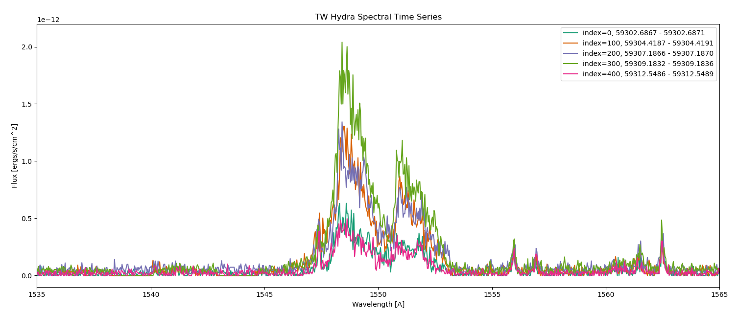
For an example of how to read in and explore these products, see the python example below.
# Import packages
from astropy.io import fits
import matplotlib.pyplot as plt

# Read in the HLSP
hlsp = "hlsp_ullyses_hst_cos_v-tw-hya_g160m_dr3_split-tss.fits"
data = fits.getdata(hlsp)
print(data.columns)
ColDefs(
    name = 'MJDSTART'; format = '440D'; unit = 'Day'
    name = 'MJDEND'; format = '440D'; unit = 'Day'
    name = 'WAVELENGTH'; format = '11562E'; unit = 'Angstrom'
    name = 'FLUX'; format = '5087280E'; unit = 'erg /s /cm**2 /Angstrom'; dim = '(11562, 440)'
    name = 'ERROR'; format = '5087280E'; unit = 'erg /s /cm**2 /Angstrom'; dim = '(11562, 440)'
)

# Examine the shapes of the data arrays
print(data["flux"][0].shape)
(440, 11562)

print(data["mjdstart"][0].shape)
(440,)

print(data["wavelength"][0].shape)
(11562,)

flux = data["flux"][0]
wavelength = data["wavelength"][0]

# Pick some random indices, and plot the spectra corresponding to those times
indices = [0, 100, 200, 300, 400]
colors = ["#1b9e77", "#d95f02", "#7570b3", "#66a61e", "#e7298a"] #colorblind-distinguishable colors
for i,ind in enumerate(indices):
    spectrum = flux[ind]
    mjdstart = data["mjdstart"][0][ind]
    mjdend = data["mjdend"][0][ind]
    plt.plot(wavelength, spectrum, color=colors[i], label=f"index={ind}, {mjdstart:.4f} - {mjdend:.4f}")
plt.legend()
plt.xlabel("Wavelength [A]")
plt.ylabel("Flux [ergs/s/cm^2]")
plt.title("TW Hydra Spectral Time Series")
plt.xlim(1535, 1565)
plt.ylim(-0.1e-12, 2.2e-12)
LCOGT Data
Observing Strategy
Photometry for ULLYSES T Tauri stars is obtained using the LCOGT 0.4m telescope network (Brown et al. 2013) which consists of ten telescopes at six observatories across the globe. For the four monitoring stars, observations are made with SDSS u' and i' filters and the Bessel V filter. For the survey stars, only the SDSS i' and Bessel V filters are used. LCOGT data are used to create spectral time-series products. DR3 includes such products for the 13 survey stars in Orion that were included in DR2. Photometry of monitoring stars and additional survey stars will be included in future data releases.Observations are planned to occur 90 and 10 days before and after the Hubble observations. These four cadences each consist of daily observations over 10-day intervals. Observations are also planned to occur during a period that encompasses the Hubble observations. For monitoring stars, 30 observations are requested over the three consecutive rotation periods being monitored. For survey stars, 10 observations are requested over the rotation period during which the Hubble observations occur. Rotation periods were estimated from TESS data and were supplied by Javier Serna (UNAM). Finally, observations are planned to occur every 15 minutes during Hubble observations.
There is not always a tight correspondence between the plans outlined above and the actual timing of observations. Weather or mechanical problems sometimes prevent observations from taking place, particularly the tightly constrained ones that are planned to run simultaneously with Hubble. In some cases, stars are not visible from any 0.4m telescope during the Hubble observations. In this release, the observations scheduled for 90 days before the Hubble observations were spread over more than the nominal 10 days as the ULLYSES team fine-tuned observing plans. A star can have more observations than expected if its field was initially used for calibration (separate calibration fields ultimately proved to be unnecessary for V and i') or if it is within a few arcsecs of another ULLYSES target.
In the event that Hubble observations fail and are rescheduled, additional LCOGT observations are scheduled to align with them. This was the case for V510 Ori, which was observed in both December 2020 and February 2021. The observations that would have been planned for 90 days after the rescheduled observations were actually constrained by the seasonal visibility of this star and instead occurred about six weeks after the rescheduled observations.
Exposure times were estimated assuming nominal sky conditions, but observations can occur during marginal sky conditions. This can result in non-detections, especially for the faintest stars in the sample.
Data Calibration
LCOGT images reduced with the BANZAI pipeline (McCully et al. 2018) are available in the LCOGT archive. BANZAI performs bad-pixel masking, bias and dark removal, and flat-field correction. It also determines the astrometric solution and extracts a catalog of sources. Using the BANZAI-reduced images, an absolute flux calibration is determined based on magnitudes cataloged by the AAVSO Photometric All-Sky Survey (APASS, funded by the Robert Martin Ayers Sciences Fund and NSF AST-1412587).The ULLYSES calibration pipeline is written in IDL. It first performs aperture photometry on sources in the BANZAI-generated catalog using aper.pro from the IDL Astronomy User's Library (Landsman 1993). It sums counts in a five-pixel radius and subtracts the modal signal in an annulus extending from 10 to 20 pixels. These sources are matched to sources in the APASS tables, using a matching radius of 2 arcsec. The relationship between APASS magnitudes and –2.5 times the logarithm of the LCOGT counts is fit with a line, ignoring three-sigma outliers. The slope of this line can vary to account for non-linearity in the instrument response; this term is typically very close to 1.
Next, the pipeline attempts to find a point source at the expected coordinates of the ULLYSES target. If a source is found, aperture photometry is performed using the same parameters described above. The measured counts are converted to a magnitude with the relationship determined above. Magnitude is then converted to a flux density using the zero-magnitude flux for the observed bandpass. Central wavelengths and zero-magnitude fluxes come from Bessell et al. 1998 for the Bessell V filter and from Fukugita et. al 1996 for the SDSS i' filter. The uncertainty is assumed to be dominated by the uncertainty in the measured counts of the ULLYSES target. Measurements with uncertainties greater than 20% of the fluxes (S/N > 5) are discarded. Output photometry files are then used as input to the spectral time-series creation code.
Targets Requiring Special Calibration
Survey T Tauri Stars
As in DR2, all STIS/G230L, G430L, and G750L data of T Tauri stars continue to require tailored calibrations. Special calibration steps taken for these observations can include: custom hot pixel identification and flagging, defringing for G750L observations, and customized spectral extraction parameters for T Tauri stars and any companions. Level 0 HLSPs (manually calibrated 1-D spectra) are provided for these stars.TW Hydra
Special calibration steps were implemented for COS spectra of the monitoring T Tauri star TW Hydra. Systematic offsets between the COS/G230L 2635 and 2950 cenwaves were corrected with a custom dispersion coefficient, or DISPTAB, reference file (available for download here). Additionally, in visit 1C the target was offset from the center of the aperture by 0.3” in cross-dispersion and 0.137” in dispersion direction. The effects of this offset were corrected using the method outlined in Section 5.3.2 of the COS Data Handbook. Finally, vignetting in the NUV channel was manually accounted for. Vignetting in COS G230L/2950 observations was corrected by scaling the stripe B continuum fluxes to those in the overlapping, temporally adjacent G230L/2635 observations.SZ10
Wavelength offsets were discovered in three visits (AC, 2D, AD) for the survey T Tauri star SZ10 and were corrected using the same method outlined for TW Hydra. Level 0 HLSPs (manually calibrated 1-D spectra) are provided for these visits.DR3 updates to HLSP Creation Code
Several updates were made to the ULLYSES HLSP creation code since DR2:- Creation of new spectral time-series HLSPs
- Creation of new imaging HLSPs
- Error counts are converted to flux using a conversion factor of flux/net counts. The code was updated such that if net counts are zero, interpolation is performed using neighboring conversion values.
- Fixed a bug where sometimes not all contributing spectra were used when coadding data. Updated products’ flux arrays will be less noisy, while error arrays will be larger or smaller by the square root of the ratio of contributing spectra before and after the bug fix.
Caveats and Known Issues
- Routine data quality checks are performed on ULLYSES HLSPs- during these checks, a region of transient elevated counts, known as a “hotspot”, was discovered on the COS/FUVB segment. This hotspot is centered at approximately X,Y=(11230, 416) with approximate extent of DX,DY=(12, 5) in RAW coordinates. The hotspot is located in one of the background regions used by CalCOS, therefore its flux is subtracted from the science spectrum resulting in a corresponding flux depression. The intensity, extent, and location of the hotspot can vary slightly with time. The exact wavelength location of the hotspot in any given spectrum will depend on the grating+FPPOS combination in use, but it is generally located between XFULL pixel 11,000 and 12,000. The earliest ULLYSES observations with this hotspot date back to November 2020, and the latest observations are as recent as August 2021. Hotspots can be identified and flagged using the appropriate COS reference file, the SPOTTAB (see Section 3.7.16 of the COS Data Handbook). Until a new SPOTTAB is delivered that accounts for it, users should be advised that this hotspot can depress flux by as little as 1e-15 to as much as 5e-14 ergs/s/cm^2/A.
- For regions where all contributing datasets have data quality issues, flux will be set to 0
- The selection of the transition wavelength from one abutted spectrum to the next is currently defined to be the middle of the overlap region. In future releases the transition wavelengths will be selected such that the signal-to-noise ratio in the input spectra at the transition wavelength is similar.
- Twenty of the T Tauri stars new to DR3 include archival data only. For these targets, while STIS/G230L, G430L, or G750L spectra exist, they are not are included in DR3. These modes require careful manual calibration, and require more time to process.
Data Description & Download
A full description of the ULLYSES data products and how they are created can be found here. Data may be downloaded from this website (HLSPs and their contributing data), the MAST Data Discovery Portal (HLSPs and their contributing data), or directly as a High-Level Science Product collection using the DOI.
Publications
A description of the ULLYSES observations and data products is given in:
For more information on how to cite ULLYSES data, see ULLYSES References.